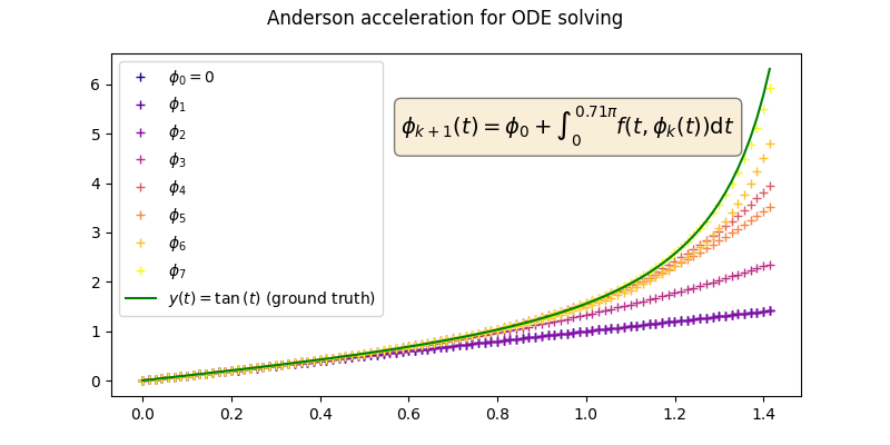
Anderson acceleration in application to Picard–Lindelöf theorem.

Thanks to the Picard–Lindelöf theorem, we can reduce differential equation solving to fixed point computations and simple integration. More precisely consider the ODE:

\[y'(t)=f(t,y(t))\]

of some time-dependant dynamic \(f:\mathbb{R}\times\mathbb{R}^d\rightarrow\mathbb{R}^d\) and initial conditions \(y(0)=y_0\). Then \(y\) is the fixed point of the following map:

\[y(t)=T(y)(t)\mathrel{\mathop:}=y_0+\int_0^t f(s,y(s))\mathrm{d}s\]

Then we can define the sequence of functions \((\phi_k)\) with \(\phi_0=0\) recursively as follows:

\[\phi_{k+1}(t)=T(\phi_k)(t)\mathrel{\mathop:} = y_0+\int_0^t f(s,\phi_k(s))\mathrm{d}s\]

Such sequence converges to the solution of the ODE, i.e., \(\lim_{k\rightarrow\infty}\phi_k=y\).

In this example we choose \(f(t,y(t))=1+y(t)^2\). We know that the analytical solution is \(y(t)=\tan{t}\) , which we use as a ground truth to evaluate our numerical scheme. We used scipy.integrate.cumtrapz to perform integration, but any other integration method can be used.

Error of 0.036270879209041595 with ground truth tan(t)

import jax
import jax.numpy as jnp

from jaxopt import AndersonAcceleration

from jaxopt import objective
from jaxopt.tree_util import tree_scalar_mul, tree_sub

import numpy as np
import matplotlib.pyplot as plt
from sklearn import datasets
from matplotlib.pyplot import cm
import scipy.integrate

jax.config.update("jax_platform_name", "cpu")


# Solve the differential equation y'(t)=1+t^2, with solution y(t) = tan(t)
def f(ti, phi):
  return 1 + phi ** 2

def T(phi_cur, ti, y0, dx):
  """Fixed point iteration in the Picard method.
  See: https://en.wikipedia.org/wiki/Picard%E2%80%93Lindel%C3%B6f_theorem"""
  f_phi = f(ti, phi_cur)
  phi_next = scipy.integrate.cumtrapz(f_phi, initial=y0, dx=dx)
  return phi_next

y0 = 0
num_interpolating_points = 100
t0 = jnp.array(0.)
tmax = 0.9 * (jnp.pi / 2) # stop before pi/2 to ensure convergence
dx = (tmax - t0) / (num_interpolating_points-1)
phi0 = jnp.zeros(num_interpolating_points)
ti = np.linspace(t0, tmax, num_interpolating_points)

sols = [phi0]
aa = AndersonAcceleration(T, history_size=5, maxiter=50, ridge=1e-5, jit=False)
state = aa.init_state(phi0, ti, y0, dx)
sol = phi0
sols.append(sol)
for k in range(aa.maxiter):
  sol, state = aa.update(phi0, state, ti, y0, dx)
  sols.append(sol)
res = sols[-1] - np.tan(ti)
print(f'Error of {jnp.linalg.norm(res)} with ground truth tan(t)')


# vizualize the first 8 iterates to make the figure easier to read
sols = sols[4:12]
fig = plt.figure(figsize=(8,4))
ax = fig.add_subplot(1, 1, 1)

colors = cm.plasma(np.linspace(0, 1, len(sols)))
for k, (sol, c) in enumerate(zip(sols, colors)):
  desc = rf'$\phi_{k}$' if k > 0 else rf'$\phi_0=0$'
  ax.plot(ti, sol, '+', c=c, label=desc)
ax.plot(ti, np.tan(ti), '-', c='green', label=r'$y(t)=\tan{(t)}$ (ground truth)')

ax.legend()
props = dict(boxstyle='round', facecolor='wheat', alpha=0.5)
formula = rf'$\phi_{{k+1}}(t)=\phi_0+\int_0^{{{tmax/2:.2f}\pi}} f(t,\phi_{{k}}(t))\mathrm{{d}}t$'
ax.text(0.42, 0.85, formula, transform=ax.transAxes, fontsize=14, verticalalignment='top', bbox=props)
fig.suptitle('Anderson acceleration for ODE solving')
plt.show()