Anderson acceleration of block coordinate descent.

Block coordinate descent converges to a fixed point. It can therefore be accelerated with Anderson acceleration.

Here m denotes the history size, and K the frequency of Anderson updates.

Bertrand, Q. and Massias, M. Anderson acceleration of coordinate descent. AISTATS, 2021.

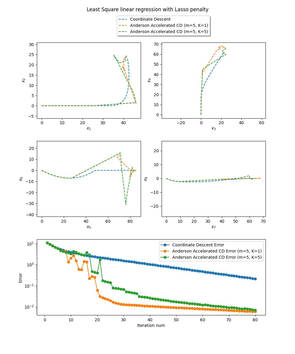
Error=0.005844 at parameters [41.41567342 24.42725366 84.7251853  65.29784113 55.85775042 -0.
  1.9099737  -0.        ] for Anderson (m=5, K=1)
Error=0.006948 at parameters [41.48824252 24.40273141 84.62864931 65.2343065  55.75704819 -0.
  1.89223564 -0.        ] for Anderson (m=5, K=5)
Error=0.210910 at parameters [41.96279774 22.87172541 82.24353772 62.41637252 52.63227623 -0.
  2.28158684 -0.        ] for Block CD

import jax
import jax.numpy as jnp

from jaxopt import AndersonWrapper
from jaxopt import BlockCoordinateDescent

from jaxopt import objective
from jaxopt import prox
from jaxopt.tree_util import tree_scalar_mul, tree_sub

import matplotlib.pyplot as plt
from sklearn import datasets

jax.config.update("jax_platform_name", "cpu")
jax.config.update("jax_enable_x64", True)


# retrieve intermediate iterates.
def run_all(solver, w_init, *args, **kwargs):
  state = solver.init_state(w_init, *args, **kwargs)
  sol = w_init
  sols, errors = [sol], [state.error]
  update = lambda sol,state: solver.update(sol, state, *args, **kwargs)
  jitted_update = jax.jit(update)
  for _ in range(solver.maxiter):
    sol, state = jitted_update(sol, state)
    sols.append(sol)
    errors.append(state.error)
  return jnp.stack(sols, axis=0), errors


X, y = datasets.make_regression(n_samples=10, n_features=8, random_state=1)
fun = objective.least_squares  # fun(params, data)
l1reg = 10.0
data = (X, y)

w_init = jnp.zeros(X.shape[1])
maxiter = 80

bcd = BlockCoordinateDescent(fun, block_prox=prox.prox_lasso, maxiter=maxiter, tol=1e-6)
history_size = 5
aa = AndersonWrapper(bcd, history_size=history_size, mixing_frequency=1, ridge=1e-4)
aam = AndersonWrapper(bcd, history_size=history_size, mixing_frequency=history_size, ridge=1e-4)

aa_sols, aa_errors = run_all(aa, w_init, hyperparams_prox=l1reg, data=data)
aam_sols, aam_errors = run_all(aam, w_init, hyperparams_prox=l1reg, data=data)
bcd_sols, bcd_errors = run_all(bcd, w_init, hyperparams_prox=l1reg, data=data)

print(f'Error={aa_errors[-1]:.6f} at parameters {aa_sols[-1]} for Anderson (m=5, K=1)')
print(f'Error={aam_errors[-1]:.6f} at parameters {aam_sols[-1]} for Anderson (m=5, K=5)')
print(f'Error={bcd_errors[-1]:.6f} at parameters {bcd_sols[-1]} for Block CD')

fig = plt.figure(figsize=(10, 12))
fig.suptitle('Least Square linear regression with Lasso penalty')
spec = fig.add_gridspec(ncols=2, nrows=3, hspace=0.3)

# Plot trajectory in parameter space (8 dimensions)
for i in range(4):
  ax = fig.add_subplot(spec[i//2, i%2])
  ax.plot(bcd_sols[:,i], bcd_sols[:,2*i+1], '--', label="Coordinate Descent")
  ax.plot(aa_sols[:,i], aa_sols[:,2*i+1], '--', label="Anderson Accelerated CD (m=5, K=1)")
  ax.plot(aam_sols[:,i], aam_sols[:,2*i+1], '--', label="Anderson Accelerated CD (m=5, K=5)")
  ax.set_xlabel(f'$x_{{{2*i+1}}}$')
  ax.set_ylabel(f'$x_{{{2*i+2}}}$')
  if i == 0:
    ax.legend(loc='upper left', bbox_to_anchor=(0.75, 1.38),
              ncol=1, fancybox=True, shadow=True)
  ax.axis('equal')

# Plot error as function of iteration num
ax = fig.add_subplot(spec[2, :])
iters = jnp.arange(len(aa_errors))
ax.plot(iters, bcd_errors, '-o', label='Coordinate Descent Error')
ax.plot(iters, aa_errors, '-o', label='Anderson Accelerated CD Error (m=5, K=1)')
ax.plot(iters, aam_errors, '-o', label='Anderson Accelerated CD Error (m=5, K=5)')
ax.set_xlabel('Iteration num')
ax.set_ylabel('Error')
ax.set_yscale('log')
ax.legend()
plt.show()